BILLONY.com Weather

How does the radar work?

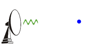
NEXRAD (Next Generation Radar) obtains weather information (precipitation and wind) based upon returned energy. The radar emits a burst of energy (green). If the energy strikes an object (rain drop, bug, bird, etc), the energy is scattered in all directions (blue). A small fraction of that scattered energy is directed back toward the radar.

This reflected signal is then received by the radar during its listening period. Computers analyze the strength of the returned pulse, time it took to travel to the object and back, and phase shift of the pulse. This process of emitting a signal, listening for any returned signal, then emitting the next signal, takes place very fast, up to around 1300 times each second.

NEXRAD spends the vast amount of time "listening" for returning signals it sent. When the time of all the pulses each hour are totaled (the time the radar is actually transmitting), the radar is "on" for about 7 seconds each hour. The remaining 59 minutes and 53 seconds are spent listening for any returned signals.

The ability to detect the "shift in the phase" of the pulse of energy makes NEXRAD a Doppler radar. The phase of the returning signal typically changes based upon the motion of the raindrops (or bugs, dust, etc.). This Doppler effect was named after the Austrian physicist, Christian Doppler, who discovered it. You have most likely experienced the "Doppler effect" around trains.

As a train passes your location, you may have noticed the pitch in the train's whistle changing from high to low. As the train approaches, the sound waves that make up the whistle are compressed making the pitch higher than if the train was stationary. Likewise, as the train moves away from you, the sound waves are stretched, lowering the pitch of the whistle. The faster the train moves, the greater the change in the whistle's pitch as it passes your location.

The same effect takes place in the atmosphere as a pulse of energy from NEXRAD strikes an object and is reflected back toward the radar. The radar's computers measure the phase change of the reflected pulse of energy which then convert that change to a velocity of the object, either toward or from the radar. Information on the movement of objects either toward or away from the radar can be used to estimate the speed of the wind. This ability to "see" the wind is what enables the National Weather Service to detect the formation of tornados which, in turn, allows us to issue tornado warnings with more advanced notice.

Is everything I see on the images an accurate picture of my weather?

Weather surveillance radars such as the WSR-88D can detect most precipitation within approximately 80 nautical miles (nm) of the radar, and intense rain or snow within approximately 140 nm. However, light rain, light snow, or drizzle from shallow cloud weather systems are not necessarily detected.

Echoes from surface targets appear in almost all radar reflectivity images. In the immediate area of the radar, "ground clutter" generally appears within a radius of 20 nm. This appears as a roughly circular region with echoes that show little spatial continuity. It results from radio energy reflected back to the radar from outside the central radar beam, from the earth's surface or buildings.

Under highly stable atmospheric conditions (typically on calm, clear nights), the radar beam can be refracted almost directly into the ground at some distance from the radar, resulting in an area of intense-looking echoes. This "anomalous propagation" phenomenon (commonly known as AP) is much less common than ground clutter. Certain sites situated at low elevations on coastlines regularly detect "sea return", a phenomenon similar to ground clutter except that the echoes come from ocean waves.

Returns from aerial targets are also rather common. Echoes from migrating birds regularly appear during nighttime hours between late February and late May, and again from August through early November. Return from insects is sometimes apparent during July and August. The apparent intensity and areal coverage of these features is partly dependent on radio propagation conditions, but they usually appear within 30 nm of the radar and produce reflectivities of <30 dBZ (decibels of Z).

However, during the peaks of the bird migration seasons, in April and early September, extensive areas of the south-central U.S. may be covered by such echoes. Finally, aircraft often appear as "point targets" far from the radar, particularly in composite reflectivity images.

The radar is also limited close in by its inability to scan directly overhead. Therefore, close to the radar, data are not available due to the radar's maximum tilt elevation of 19.5¡. This area is commonly referred to as the radar's "Cone of Silence".

Though surface echoes appear in the base and composite reflectivity images, special automated error checking generally removes their effects from precipitation accumulation products. The national reflectivity mosaic product is also automatically edited to detect and remove most nonprecipitation features. Even with limited experience, users of unedited products can differentiate precipitation from other echoes, if they are aware of the general meteorological situation.

What are the different types of radar images?

Base Reflectivity

This is a display of echo intensity (reflectivity) measured in dBZ (decibels of Z, where Z represents the energy reflected back to the radar). "Reflectivity" is the amount of transmitted power returned to the radar receiver. Base Reflectivity images are available at several different elevation angles (tilts) of the antenna and are used to detect precipitation, evaluate storm structure, locate atmospheric boundaries and determine hail potential.

The base reflectivity image currently available on this website is from the lowest "tilt" angle (0.5¡). This means the radar's antenna is tilted 0.5¡ above the horizon.

The maximum range of the "short range" (S Rng) base reflectivity product is 124 nm (about 143 miles) from the radar location. This view will not display echoes that are more distant than 124 nm, even though precipitation may be occurring at greater distances. To determine if precipitation is occurring at greater distances, select the "long range" (L Rng) view (out to 248 nm/286 mi), select an adjacent radar, or link to the National Reflectivity Mosaic.

Composite Reflectivity

This display is of maximum echo intensity (reflectivity) from any elevation angle at every range from the radar. This product is used to reveal the highest reflectivity in all echoes. When compared with Base Reflectivity, the Composite Reflectivity can reveal important storm structure features and intensity trends of storms.

The maximum range of the "long range" (L Rng) composite reflectivity product is 248 nm (about 286 miles) from the radar location. The "blocky" appearance of this product is due to its lower spatial resolution on a 2.2 * 2.2 nm grid. It has one-fourth the resolution of the Base Reflectivity and one-half the resolution of the Precipitation products.

Although the Composite Reflectivity product is able to display maximum echo intensities 248 nm from the radar, the beam of the radar at this distance is at a very high altitude in the atmosphere. Thus, only the most intense convective storms and tropical systems will be detected at the longer distances.

Because of this fact, special care must be taken interpreting this product. While the radar image may not indicate precipitation it's quite possible that the radar beam is overshooting precipitation at lower levels, especially at greater distances. To determine if precipitation is occurring at greater distances link to an adjacent radar or link to the National Reflectivity Mosaic.

For a higher resolution (1.1 * 1.1 nm grid) composite reflectivity image, select the short range (S Rng) view. The image is less "blocky" as compared to the long range image. However, the maximum range is reduced to 124 nm (about 143 miles) from the radar location.

One-hour Precipitation

This is an image of estimated one-hour precipitation accumulation on a 1.1 nm by 1 degree grid. This product is used to assess rainfall intensities for flash flood warnings, urban flood statements and special weather statements. The maximum range of this product is 124 nm (about 143 miles) from the radar location. This product will not display accumulated precipitation more distant than 124 nm, even though precipitation may be occurring at greater distances. To determine accumulated precipitation at greater distances you should link to an adjacent radar.

Storm Total Precipitation

This image is of estimated accumulated rainfall, continuously updated, since the last one-hour break in precipitation. This product is used to locate flood potential over urban or rural areas, estimate total basin runoff and provide rainfall accumulations for the duration of the event.

The maximum range of this product is 124 nm (about 143 miles) from the radar location. This product will not display accumulated precipitation more distant than 124 nm, even though precipitation may be occurring at greater distances. To determine accumulated precipitation at greater distances link to an adjacent radar.

How often are the images updated?

Image updates are based upon the operation mode of the radar at the time the image is generated. The WSR-88D Doppler radar is operated in one of two modes -- clear air mode or precipitation mode. In clear air mode, images are updated every 10 minutes. In precipitation mode, images are updated every four to six minutes. The collection of radar data, repeated at regular time intervals, is referred to as a volume scan.

In this mode, the radar is in its most sensitive operation. This mode has the slowest antenna rotation rate which permits the radar to sample a given volume of the atmosphere longer. This increased sampling increases the radar's sensitivity and ability to detect smaller objects in the atmosphere than in precipitation mode. A lot of what you will see in clear air mode will be airborne dust and particulate matter. Also, snow does not reflect energy sent from the radar very well. Therefore, clear air mode will occasionally be used for the detection of light snow.

The radar continuously scans the atmosphere by completing volume coverage patterns (VCP). A VCP consists of the radar making several 360¡ scans of the atmosphere, sampling a set of increasing elevation angles. There are two clear mode VCPs.

In clear air mode, the radar begins a volume scan at the 0.5¡ elevation angle (i.e., the radar antenna is angled 0.5¡ above the ground). Once it makes two full sweeps (a surveillance/reflectivity sweep and a Doppler/velocity sweep) at the 0.5¡ elevation angle, it increases to 1.5¡ and makes two more 360¡ rotations. For one of the clear air mode VCPs, two full sweeps are also made at 2.5¡. Otherwise, at the higher elevations (2.5¡, 3.5¡, and 4.5¡) a single sweep is made (reflectivity and velocity data are collected together).

This process is repeated at 2.5¡, 3.5¡, and 4.5¡. Then the radar returns to the 0.5¡ elevation angle to begin the next volume scan which will repeat the same sequence of elevation angles. In clear air mode, the complete scan of the atmosphere takes about 10 minutes at 5 different elevation angles.

When precipitation is occurring, the radar does not need to be as sensitive as in clear air mode as rain provides plenty of returning signals. At the same time, meteorologists want to see higher in the atmosphere when precipitation is occurring to analyze the vertical structure of the storms. This is when the meteorologists switch the radar to precipitation mode using one of two volume coverage patterns.

Both precipitation VCP's begin like the clear air mode mentioned above with the same evaluations scans as in the clear air mode. The difference is the radar continues looking higher in the atmosphere, up to 19.5¡ to complete the volume scan. The time it takes to complete the entire volume scan is also less. In the slower VCP, the radar completes the volume scan of nine different elevations in six minutes. In the faster VCP, the radar completes 14 different elevation scans in five minutes.

Differences in the quality of radar images between the two precipitation mode VCPs are relatively minor. Therefore, during severe weather, the faster VCP is almost always used as it provides the meteorologists with the quickest updates and most elevation slices through the storms.

In summary, when the radar is in clear air mode, radar images will be updated approximately every ten minutes. In precipitation mode, the updates will occur around five to six minutes apart.

What do the colors mean in the reflectivity products?

The colors are the different echo intensities (reflectivity) measured in dBZ (decibels of Z) during each elevation scan. "Reflectivity" is the amount of transmitted power returned to the radar receiver. Reflectivity (designated by the letter Z) covers a wide range of signals (from very weak to very strong). So, a more convenient number for calculations and comparison, a decibel (or logarithmic) scale (dBZ), is used.

dBZ	Rainrate  (in/hr)
65	16+
60	8.00
55	4.00
52	2.50
47	1.25
41	0.50
36	0.25
30	0.10
20	Trace

The dBZ values increase as the strength of the signal returned to the radar increases. Each reflectivity image you see includes one of two color scales. One scale (far left) represents dBZ values when the radar is in clear air mode (dBZ values from -28 to +28). The other scale (near left) represents dBZ values when the radar is in precipitation mode (dBZ values from 5 to 75). Notice the color on each scale remains the same in both operational modes, only the values change. The value of the dBZ depends upon the mode the radar is in at the time the image was created.

The scale of dBZ values is also related to the intensity of rainfall. Typically, light rain is occurring when the dBZ value reaches 20. The higher the dBZ, the stronger the rainrate. Depending on the type of weather occurring and the area of the U.S., forecasters use a set of rainrates which are associated to the dBZ values.

These values are estimates of the rainfall per hour, updated each volume scan, with rainfall accumulated over time. Hail is a good reflector of energy and will return very high dBZ values. Since hail can cause the rainfall estimates to be higher than what is actually occurring, steps are taken to prevent these high dBZ values from being converted to rainfall.

What is the difference between base and composite reflectivity?

The main difference is composite reflectivity shows the highest dBZ (strongest reflected energy) at all elevation scans, not just the reflected energy at a single elevation scan. This can be seen in the images below from the Salt Lake City radar.

	Base Reflectivity		Composite Reflectivity

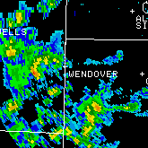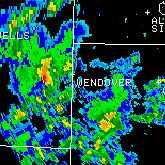Notice the additional reflectivity that is visible in the composite reflectivity (far right). It is most readily seen around the name 'Wendover'. Also notice the composite view displays a slightly larger area of heavy rain (orange-red area to the west of Wendover).

Why the difference? Base reflectivity only shows reflected energy at a single elevation scan of the radar. Composite reflectivity displays the highest reflectivity of ALL elevations scans. So, if heavier precipitation is higher in the atmosphere over an area of lighter precipitation (the heavier rain that has yet to reach the ground), the composite reflectivity image will display the stronger dBZ level.

This occurs often with severe thunderstorms. The updraft, which feeds the thunderstorm with moist air, is strong enough to keep a large amount of water aloft. Once the updraft can no longer support the weight of suspended water then the rain intensity at the surface increases as the rain falls from the cloud.

What is UTC Time?

	Standard Time									Daylight Saving
UTC	Guam	HI	AK	PST	MST	CST	EST	AST		PDT	MDT	CDT	EDT
Diff	+10	-10	-9	-8	-7	-6	-5	-4		-7	-6	-5	-4
00	10a	2p*	3p*	4p*	5p*	6p*	7p*	8p*		5p*	6p*	7p*	8p*
01	11a	3p*	4p*	5p*	6p*	7P*	8p*	9p*		6p*	7p*	8p*	9p*
02	12N	4p*	5p*	6p*	7p*	8p*	9p*	10p*		7p*	8p*	9p*	10p*
03	1p	5p*	6p*	7p*	8p*	9p*	10p*	11p*		8p*	9p*	10*	11p*
04	2p	6p*	7p*	8p*	9p*	10p*	11p*	12M		9p*	10p*	11p*	12M
05	3p	7p*	8p*	9p*	10p*	11p*	12M	1a		10p*	11p*	12M	1a
06	4p	8p*	9p*	10p*	11p*	12M	1a	2a		11p*	12M	1a	2a
07	5p	9p*	10p*	11p*	12M	1a	2a	3a		12M	1a	2a	3a
08	6p	10p*	11p*	12M	1a	2a	3a	4a		1a	2a	3a	4a
09	7p	11p*	12M	1a	2a	3a	4a	5a		2a	3a	4a	5a
10	8p	12M	1a	2a	3a	4a	5a	6a		3a	4a	5a	6a
11	9p	1a	2a	3a	4a	5a	6a	7a		4a	5a	6a	7a
12	10p	2a	3a	4a	5a	6a	7a	8a		5a	6a	7a	8a
13	11p	3a	4a	5a	6a	7a	8a	9a		6a	7a	8a	9a
14	12M%	4a	5a	6a	7a	8a	9a	10a		7a	8a	9a	10
15	1a%	5a	6a	7a	8a	9a	10a	11a		8a	9a	10a	11a
16	2a%	6a	7a	8a	9a	10a	11a	12N		9a	10a	11a	12N
17	3a%	7a	8a	9a	10a	11a	12N	1p		10a	11a	12N	1p
18	4a%	8a	9a	10a	11a	12N	1p	2p		11a	12N	1p	2p
19	5a%	9a	10a	11a	12N	1p	2p	3p		12N	1p	2p	3p
20	6a%	10a	11a	12N	1p	2p	3p	4p		1p	2p	3p	4p
21	7a%	11a	12N	1p	2p	3p	4p	5p		2p	3p	4p	5p
22	8a%	12N	1p	2p	3p	4p	5p	6p		3p	4p	5p	6p
23	9a%	1p	2p	3p	4p	5p	6p	7p		4p	5p	6p	7p
AST - Atlantic, AK - Alaska time, HI - Hawaii time, *The previous day, %The next day

Weather observations around the world (including radar observations) are always taken with respect to a standard time. By convention, the world's weather communities use a twenty four hour clock, similar to "military" time based on the 0¡ longitude meridian, also known as the Greenwich meridian.

Prior to 1972, this time was called Greenwich Mean Time (GMT) but is now referred to as Coordinated Universal Time or Universal Time Coordinated (UTC). It is a coordinated time scale, maintained by the Bureau International des Poids et Mesures (BIPM). It is also known a "Z time" or "Zulu Time".

To obtain your local time here in the United States, you need to subtract a certain number of hours from UTC depending on how many time zones you are away from Greenwich (England). The table (right) shows the standard difference from UTC time to local time.

The switch to daylight saving time does not affect UTC. It refers to time on the zero or Greenwich meridian, which is not adjusted to reflect changes either to or from Daylight Saving Time.

However, you need to know what happens during daylight saving time in the United States. In short, the local time is advanced one hour during daylight saving time. As an example, the Eastern Time zone difference from UTC is a -4 hours during daylight saving time rather than -5 hours as it is during standard time.

From National Weather Service